So k-NNs tend to work well until we start adding more and more variables, where the input space becomes more and more sparsely populated. And once we begin to suspect that certain variables are less or more relevant or lie on a different scale from others, we have another problem on our hands: defining distance.
Now’s a good time to step back and think about what exactly the k-NN algorithm does. The k-NN algorithm merely compares new data to the old data; but is that what we do to learn?
Probably not. Recall from lesson one when we were trying to figure out how to define artificial intelligence: we were picking out a common trait to every AI problem that would distinguish it from a simple computational problem.
Rules from Data
When we learn with intent, we look for patterns. We take provided data and igure out what information is relevant and what to throw out. You can recognize a digit by its shape, but not so much from its typeface or medium.
So that’s exactly what we should do: finding rules from data is simply about picking out the relevant information to use given the data.
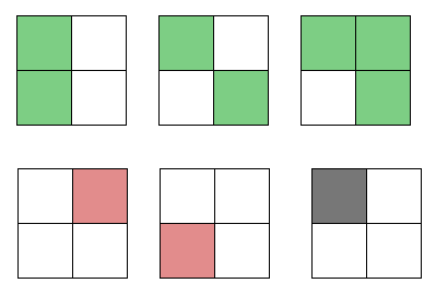
To see how we’d approach this, let’s play with some toy data. Should the unclassified (black) data point be classified red or green?
Take a moment to think about it. What rule does the sample data seem to fall into, and what would that imply for the new data point?
If you said green, you’re right! All the green-classified bocks have the top-left square filled in.
If you said red, you’re… also right! All the red-classified blocks have only one square filled in.
Wait a second.
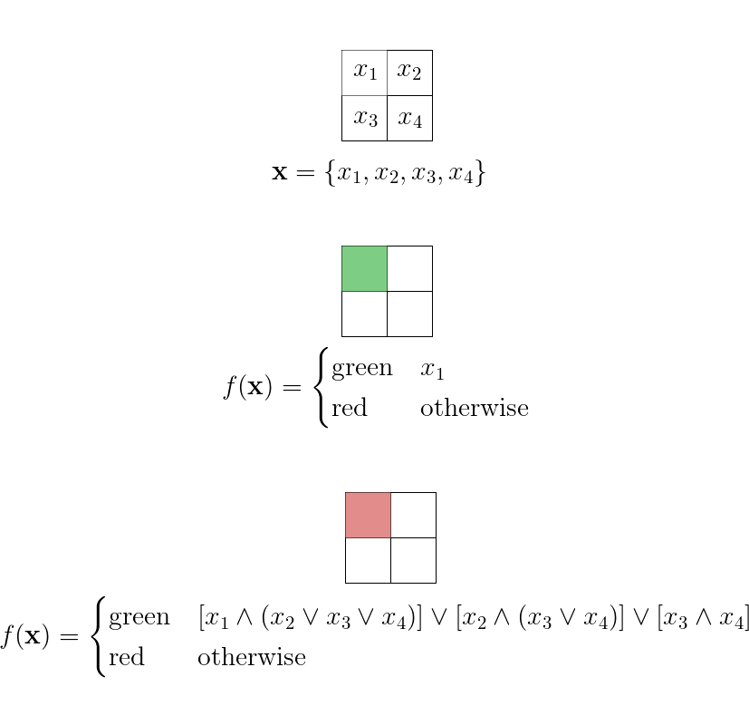
Okay, there seems to be multiple rules that might work; so how about we try to enumerate all distict rules that might work for this set of sample data? To be precise, we can label each square of a block with a boolean variable and then we’re just tring to find an \(f:\mathbb{B}^4\mapsto\{\text{red},\text{green}\}\)[1] that works with the sample data.
 [2]
[2]
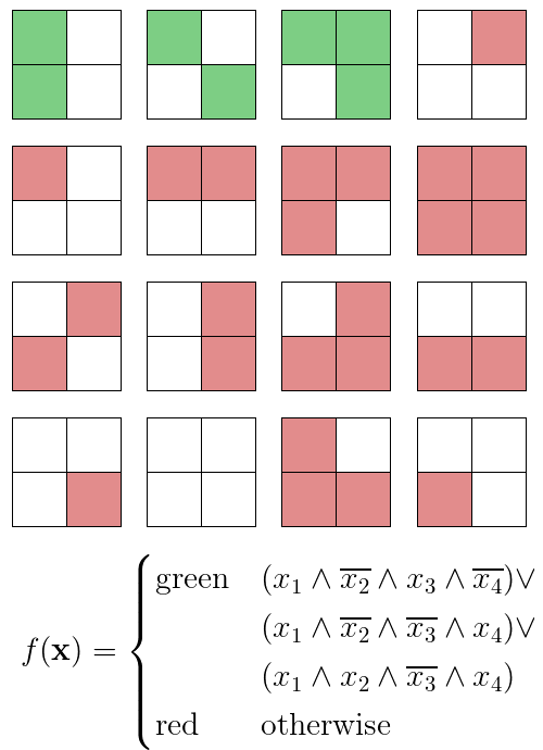
Alright; well, let’s first try to break this approach. Is there a way to tailor our rule so that every input is classified red except for the three green-classified sample blocks?
 [3]
[3]
Oh.
There are \(2^4=16\) possible, distinct blocks. If our function can be tailored for individiual blocks, then all eleven blocks that we haven’t yet classified could go either way for any given rule. Then, we’d have \(2^{11}=2048\) distinct rules that fit the sample toy data.
We can’t resolve this easily, either; if we tried something like democracy, where every rule gets a vote for each new data point, we still wouldn’t get anywhere, since half the rules would classify red and the other half green.
We can’t just learn rules from data. There’s no real rational basis to choose one rule over another.
And this brings us to our second pillar of machine learning:
Machine Learning is fundamentally ill-posed.
Bias and Variance
We’ve just found that learning rules from data seems to be meaningless. What now?
Recall from our development of the k-NN algorithm one of the pillars of machine learning we stumbled upon: to learn is to generalize. Here,wWe’re going to do something that makes most good mathematicians uncomfortable: we’re going to make an assumption.
The key assumption to make here is that the simple rules are better; after all, the more general a rule, the more simple its formulation must be.
Is this assumption problematic? It could be; after all, the point of an assumption is to throw away possibiliites that seem like they won’t work out.
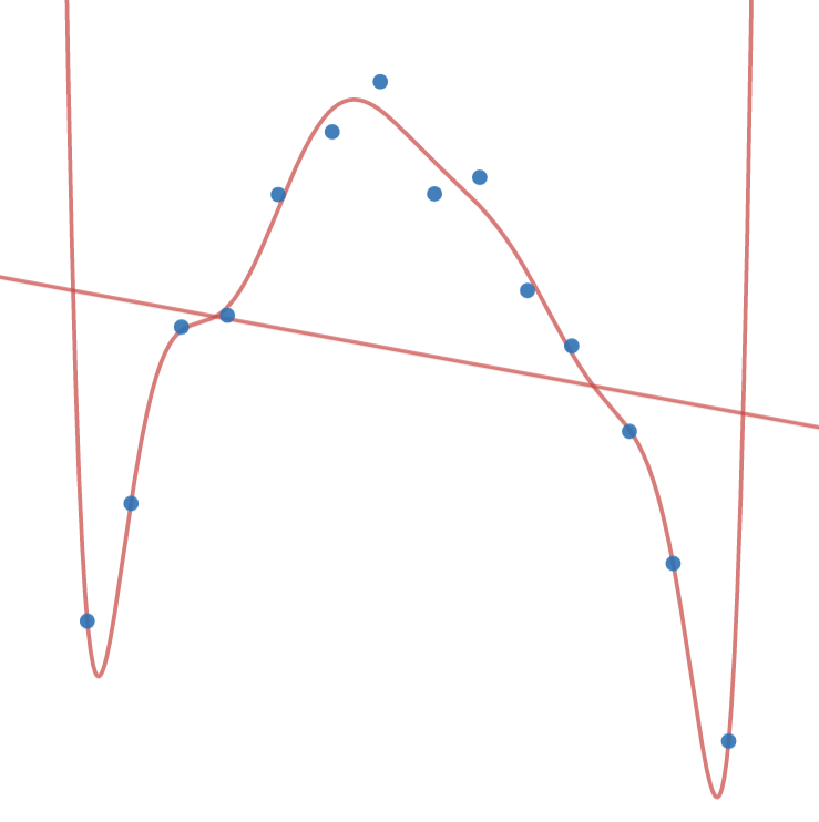
But there’s a good argument for this assumption. Sample data is pulled from the perhaps-infinite pool of real, possible data to use. While overly-simple rules might not be expressive enough to truly classify our data, that can be detected from tests against our sample data. However, the more expressive we let our rules be, the more and more likely any rule we test will match the sample data by luck alone. At a certain point of complexity, we’re practically guaranteeing that we’ll find many rules that perfectly match our sample data, finding patterns in the sample data that doesn’t exit in general. And once that’s occurred, we’ve overfit our data — we’ve given up on looking for a meaningful, general pattern and are merely trying to find a perfect function for our noisy data. The better we do on our training data, the more likely we’re overfitting.
The opposite, of course, is underfitting with rules that are too general. The closer the performance between the training and real data, the more likely we’re underfitting.
Here we reach our third pillar of machine learning:
<span id="L1" class="line">Machine learning algorithms must both perform well on training data and generalize,</span>
<span id="L2" class="line">two goals which are fundamentally opposed.</span>
Use rules that are too simple, that have too much bias, and we risk underfitting. Use rules that are too expressive, that have too much variance, and we risk overfitting. How do we deal with this?
Underfitting can be detected when we try to run through the AI the data we trained it with: if it does poorly on the data it had been trained with, then our rules are obviously not expressive enough to describe the data. And simiarly, overfitting can be detected when we run new data through the AI: if there’s a large drop in performance from the training data, then our AI has found patterns in the training data that exist only by coincidence.
What we can do then is split the provided data into a set of training data and a set of testing data; we’ll use the training data to learn rules and test those rules against the testing data to prevent overfitting.
Let’s do a thought experiment with the MNIST data. For the sake of simplicity, for now we’ll just work with classifying images as images of a zero or not of a zero.
We’ll begin with the most simple, more general, most biased type of rule: the zero-pixel rule. We’ll take the best zero-pixel rule to decide whether or not the picture is a zero.
As you can expect, this would perform exceptionally poorly. All pictures would be blanket-designated "not a zero." But it’s a very general rule, and its performance is the same across both training and testing data.
But it’s too biased, so we should crank up the variance. There are \(28^2\cdot2=1568\) one-pixel rules to choose form the check fro zero-ness. Now, a one-pixel rule is probably a bit too biased, which we’d be able to see from its performance on the training data, so we’ll slowly increase the variance until the losses on the testing data begin to take over.
We’ve searched through the two zero-pixel rules and fifteen-hundred one-pixel rules, and we’ll search through the \(\binom{28^2}{2}\cdot2^2=1\,227\,744\) two-pixel rules, \(\binom{28^2}{3}\cdot2^3=640\,063\,872\) three-pixel rules, \(\binom{28^2}{4}\cdot2^4=249\,944\,942\,016\) four-pixel rules until we get to the one that’ll work best.
Wait a second.
By the time we’re looking for the best four-pixel rule, we’re already dealing with two hundred billion rules. If we could evaluate one million rules every second, just looking for the best four-pixel rule would take two days and twenty-one and a half hours to compute.
But this isn’t really a problem, right? We can be patient; we’ll have time to fix this after we’ve conquered the world with machine learning, after all.
The search for the best five-pixel rule would take two and a half years. The best six will take over six centuries. Ten would take about fifty-four times the age of the universe.
Obviously, this is kind of problematic. The number of rules we need to test rapidly increases, and the growth is quickly unsustainable.
This problem of having unbelievably fast growth in computational complexity wiht just small increases in the input is called intractability. And despite years of research, problems of this type still have no reasonably-growing solutions. Intractability is responsible for an AI winter of its own, and it wasn’t for a while until some developments allowed us to work around it.