So having people come up with rules is too expensive. Instead, we should consider making machines themselves come up with rules.
How?
Bashing Your Head at a Problem
Once again, we can try and use a brute-force approach. Our goal is to make a machine "learn" rules from sample data.

One very, very simple way to do this is to just make the sample data the rules. If you get an input that exactly matches that of one of the sample data, we’re done! Obviously the result should match the label of the datapoint in the sample.
On the right is a sample of the MNIST database. The entire database is, of course, much larger.
But I think we can already start to see a problem.
There’s way, way too much variation among individual digits. And even if you tried to write a single digit in exactly the same way, you wouldn’t get it to pixel-perfect intensity.
This is memorization.
One datapoint in the MNIST dataset consists of the digit that was intended to be written, and a twenty-eight by twenty-eight grayscale image of the written digit. In other words, there’s \(256^{28\times 28}\), or about \(1.15\times10^{1888}\) distinct images to consider.
There are about \(10^{80}\) atoms in the visible universe.
To memorize not to learn.
We certainly don’t compare every digit we see to every digit we’ve seen previously to try and find a match. When we learn language, we don’t memorize every sentence that appears.
No, we look for patterns. In language, we look for patterns in the usage of words — vocabulary — and in the placement of words — grammar. We look for simpler rules, and for generalizations.
And here, we arrive at one of the pillars of machine learning, an aphorism that extends beyond academia:
To learn is to generalize.
Similarities
So how do we generalize?
After just a little bit of thought, it may seem obvious that we should look for whichever sample data is most similar to the input. And this is quite a reasonable thing to do.
In fact, it’s such a reasonable thing to do that computer scientists call it nearest neighbour search.
The opposite of a similarity is a difference, and looking for the most similar is equivalent to finding the least different. If you have prior knowledge of statistics, you’ll know that differences are easier to quantify and measure, which is why we’ll use that too.
If we considered a very, very simple problem to put it against, we can see how this works. Consider if we had toy data for a two-variable binary classification — that is, we know two pieces of information, and we’ll use that to decide whether that should result in yes it is/no it isn’t classification.
You may notice that this could be an extremely simplified version of digit classification: with MNIST, there were \(28^2=784\) different pixels, ie. pieces of information per data point, and ten different classifications. Simplifying problems into something easily manageable is a common technique, and will be an immense aid in understanding.
In the toy data, we had only two different variables, which give rise to a simple binary classification. If you recall from basic statistics classes in grade school where you called the subject "data management," you’ll recall that you can plot two-variable data points on a two-dimensional scatter plot.
From there, the difference — or "inverse similarity" if you’d prefer — between two data points is just the distance between them. By Pythagoras,
Of course, if your two variables have very different scales — like a country’s GDP per capita[1] compared to its rating on the Democracy Index[2] — the distance formula would have to be adjusted or the variable with larger range would be too highly-favoured.
From there, every new input just needs their distance against every training data point computed, and the resulting classification is the same as that of the closest training data point.
Extending this back to a larger number of variables and classifications is trivial; the distance formula simply becomes the general \(n\)-dimensional distance formula:
... and the resulting classification is still the same as that of the least-distant training data point.


And I think that by comparing the above two images here, you can immediately see some problems with this approach.
Simplicity
You can see one the left-hand-side image that there’s three large clusters of red, green, and blue. There are some elements of another colour sort of "infiltrating" these clusters, but this can simply be due to mislabeled sample data or ambiguous cases — training data is pre-labeled, usually by humans, after all.[4]
Every data point is not equal. Some are outliers, and that must be dealt with.
There’s one tiny, easy change we can make here. Our previous approach was to find the nearest neighbour. The title of this lesson is k-nearest neighbours.
The k-Nearest Neighbour algorithm isn’t particulary flashy or modern — it was in use by 1967 — but it’s our first step into making a real machine-learning algorithm. And the improvement from the basic nearest-neighbour algorithm is quite impressive:
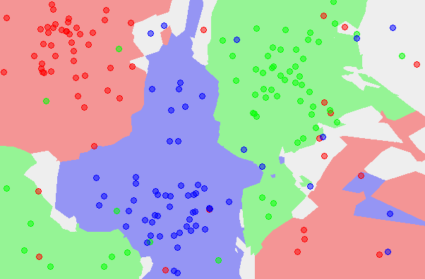
On the left is the old nearest-neighbour (NN) output space; on the right is the 5-nearest-neighbours (5-NN) output space. And you can see how it cleanly separates the clusters with few exceptions, and that it recognizes spaces that may be ambiguous due to the lack of data.
Today, the k-NN approach is a common first line of attack for machine-learning problems; many applications don’t need anything more complicated.
So let’s get back to working with the MNIST database. There’s a few problems with using a bare k-NN approach, but we can improve its performance with a few techniques such as slightly blurring out the images. And after doing so, it can achieve a 3-4% error rate.
And that’s quite impressive for a problem that we’d never figure out through an expert system approach.
So it looks like we’ve figured out machine learning, huh?
Not at all.
There are still many problems with the k-Nearest Neighbours approach. You can already see in the 5-NN output space above that in areas with sparse data, there will still be many glitches. You can also see that although the algorithm generalizes well for large, clear clusters, it doesn’t for small, local clusters — and in the areas without much data, it still gives biazarre boundaries. The k-NN approach both overfits and underfits at the same time.[5]
And finally, when we try to apply it to the MNIST database, we can see another problem. Each data point contains too much data. There are seven-hundred-eighty-four different dimensions.
Twenty-eight by twenty-eight is a tiny picture. What will happen when we try to do it with 256x256 pictures?
K-Nearest Neighbours is a good approach to start with, but we need something better.